Stock Buy Sell Algorithm: Multiple Transaction with Codes

Sasank is a Technical Content Writer with a strong background in competitive programming. He has solved nearly 1500 problems on LeetCode and achieved top rankings in LeetCode Weekly Contests, including global ranks of 171, 196, 206, 308, 352, and more. His expertise in algorithms and problem-solving is also reflected in his active participation on platforms like Codeforces. Sasank enjoys sharing his technical knowledge and helping others learn by creating clear and accessible content.


Problem Statement
You are given an array of integers representing stock prices on consecutive days. Your task is to find the maximum profit you can make by buying and selling stocks. You can make multiple transactions (buy one share, sell it, then buy again), but you must sell the stock before buying it again - meaning you can only hold at most one share at any time.
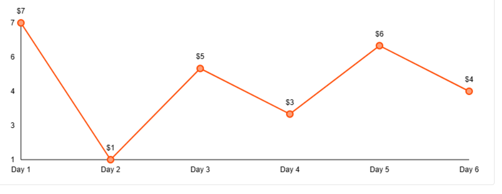
For example, if the stock prices are [7, 1, 5, 3, 6, 4], the maximum profit would be 7 (buy at 1, sell at 5, buy at 3, sell at 6).
Brute Force Approach
Explanation
The brute force approach considers all possible combinations of buying and selling days. For each day, we have three choices:
- Buy a stock (if we don't already own one)
- Sell a stock (if we own one)
- Do nothing
We try all possible sequences of these actions and find the one that gives the maximum profit.
This approach, while conceptually simple, becomes extremely inefficient as the number of days increases due to the exponential number of possibilities.
Time Complexity: O(3^n) where n is the number of days
Space Complexity: O(n) for the recursion stack
Code (Python)
def max_profit_brute_force(prices):
    def recursive_profit(index, can_buy):
        # Base case: reached the end of the array
        if index >= len(prices):
            return 0

        # Do nothing option
        do_nothing = recursive_profit(index + 1, can_buy)

        if can_buy:
            # Buy option: subtract price and can't buy again
            buy = recursive_profit(index + 1, False) - prices[index]
            return max(do_nothing, buy)
        else:
            # Sell option: add price and can buy again
            sell = recursive_profit(index + 1, True) + prices[index]
            return max(do_nothing, sell)

    # Start with day 0 and ability to buy
    return recursive_profit(0, True)
Code (C++)
#include <vector>
#include <algorithm>
using namespace std;

class Solution {
public:
    int maxProfit(vector<int>& prices) {
        return recursiveProfit(prices, 0, true);
    }

private:
    int recursiveProfit(vector<int>& prices, int index, bool canBuy) {
        // Base case: reached the end of the array
        if (index >= prices.size()) {
            return 0;
        }

        // Do nothing option
        int doNothing = recursiveProfit(prices, index + 1, canBuy);

        if (canBuy) {
            // Buy option: subtract price and can't buy again
            int buy = recursiveProfit(prices, index + 1, false) - prices[index];
            return max(doNothing, buy);
        } else {
            // Sell option: add price and can buy again
            int sell = recursiveProfit(prices, index + 1, true) + prices[index];
            return max(doNothing, sell);
        }
    }
};
Code (Java)
class Solution {
    public int maxProfit(int[] prices) {
        return recursiveProfit(prices, 0, true);
    }

    private int recursiveProfit(int[] prices, int index, boolean canBuy) {
        // Base case: reached the end of the array
        if (index >= prices.length) {
            return 0;
        }

        // Do nothing option
        int doNothing = recursiveProfit(prices, index + 1, canBuy);

        if (canBuy) {
            // Buy option: subtract price and can't buy again
            int buy = recursiveProfit(prices, index + 1, false) - prices[index];
            return Math.max(doNothing, buy);
        } else {
            // Sell option: add price and can buy again
            int sell = recursiveProfit(prices, index + 1, true) + prices[index];
            return Math.max(doNothing, sell);
        }
    }
}
Optimized Approach
Explanation
The key insight for optimizing this problem is to notice that the maximum profit comes from capturing every upward price movement. Since we can make multiple transactions, we should buy before every price increase and sell after it.
For example, if prices increase from day 1 to day 2, we should buy on day 1 and sell on day 2. This approach gives us a simple algorithm: add up all positive price differences between consecutive days.
Time Complexity: O(n) where n is the number of days
Space Complexity: O(1) - we only need a few variables
Lets Consider array [7 1 5 3 6 4]
i = 1:
- Compare: prices[1] = 1 vs prices[0] = 7
- 1 is not greater than 7 → no profit
→ max_profit = 0
i = 2:
- Compare: prices[2] = 5 vs prices[1] = 1
- 5 > 1 → Buy at 1, sell at 5 → profit = 4
→ max_profit = 0 + 4 = 4
i = 3:
- Compare: prices[3] = 3 vs prices[2] = 5
- 3 is not greater than 5 → no profit
→ max_profit = 4
i = 4:
- Compare: prices[4] = 6 vs prices[3] = 3
- 6 > 3 → Buy at 3, sell at 6 → profit = 3
→ max_profit = 4 + 3 = 7
i = 5:
- Compare: prices[5] = 4 vs prices[4] = 6
- 4 is not greater than 6 → no profit
→ max_profit = 7
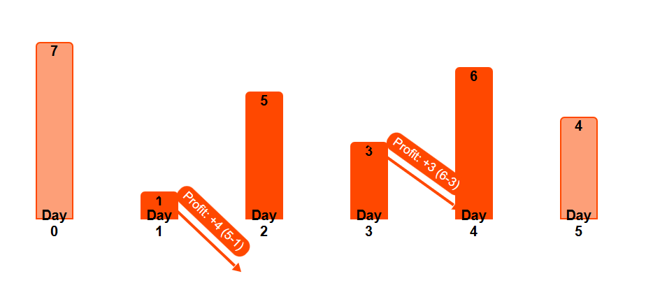
Therefore total profit is 4 + 3 = 7.
Stock Buy Sell Algorithm Visualization
<visualization-box>
Code (Python)
def max_profit_optimized(prices):
    max_profit = 0

    # Loop through adjacent pairs
    for i in range(1, len(prices)):
        # If current price is higher than previous day's price
        if prices[i] > prices[i - 1]:
            # Add the price difference to our profit
            max_profit += prices[i] - prices[i - 1]

    return max_profit
Code (C++)
#include <vector>
using namespace std;

class Solution {
public:
    int maxProfit(vector<int>& prices) {
        int maxProfit = 0;

        // Loop through adjacent pairs
        for (int i = 1; i < prices.size(); i++) {
            // If current price is higher than previous day's price
            if (prices[i] > prices[i - 1]) {
                // Add the price difference to our profit
                maxProfit += prices[i] - prices[i - 1];
            }
        }

        return maxProfit;
    }
};
Code (Java)
class Solution {
    public int maxProfit(int[] prices) {
        int maxProfit = 0;

        // Loop through adjacent pairs
        for (int i = 1; i < prices.length; i++) {
            // If current price is higher than previous day's price
            if (prices[i] > prices[i - 1]) {
                // Add the price difference to our profit
                maxProfit += prices[i] - prices[i - 1];
            }
        }

        return maxProfit;
    }
}
Conclusion
We tackled the multiple-transaction stock buy and sell problem using two approaches:
1. A brute force approach that explores all possible buying and selling combinations, which is conceptually clear but inefficient with O(3^n) time complexity.
2. An optimized approach that simply captures all upward price movements, resulting in O(n) time complexity.
The stark contrast between these approaches illustrates an important programming lesson: sometimes complex problems have surprisingly elegant solutions. The optimized solution here doesn't require any advanced data structures or algorithms - just a key insight about the problem.