Arrays: Essential Operations & Implementation Guide

Written by

Sasank Nasika

Edited by

Raj Aryan

Last updated on

May 10, 2025

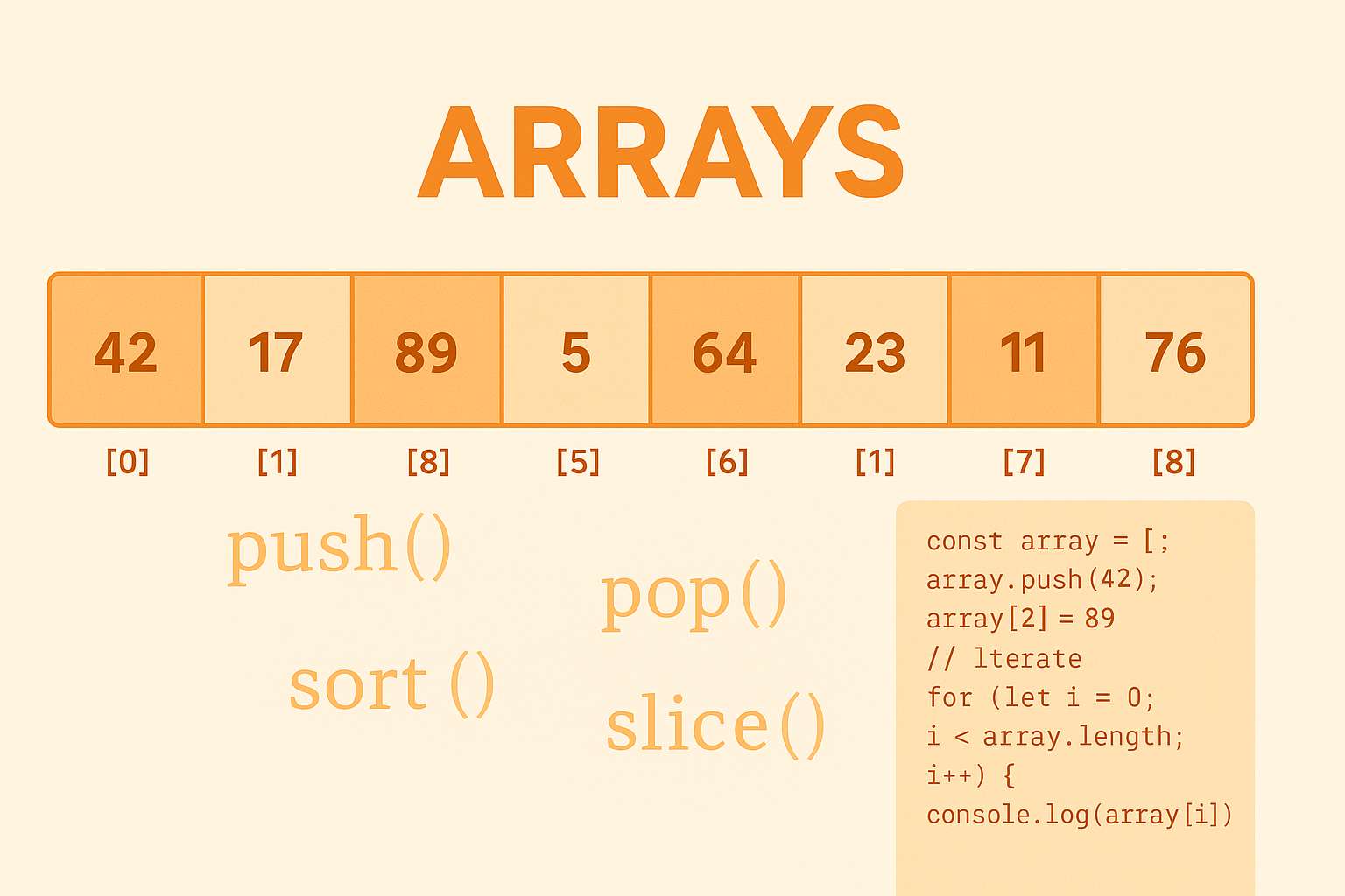
Arrays are fundamental data structures in programming that store collections of items of the same type. They act as containers holding multiple values under a single variable name, with each value accessible through an index. Arrays form the foundation for many complex applications and algorithms in computer science.

Arrays: Essential Operations & Implementation Guide

Array Fundamentals

Characteristics of Arrays

Homogeneous Elements

Arrays store elements of the same data type. This uniformity allows the computer to calculate the exact memory location of any element in constant time. For example, in an integer array, each element must be an integer; you cannot mix integers with strings or other data types in the same array.

# Valid array of integers

numbers = [1, 2, 3, 4, 5]

# Valid array of strings

names = ["Resume Builder", "Interview Copilot", "FinalRoundAI"]

# This would be invalid in strictly typed languages:

# mixed = [1, "hello", 3.14]

Contiguous Memory Allocation

A key property of arrays is that elements are stored in adjacent memory locations. This contiguous allocation enables quick access to any element using its index.

Types of Arrays

One-dimensional Arrays

The simplest form of arrays contains elements arranged in a linear sequence. Each element is accessed using a single index.

Python

numbers = [42, 17, 89, 36, 23, 64]; print(numbers[2]) # Outputs: 89

C++

int numbers[] = {42, 17, 89, 36, 23, 64}; cout << numbers[2] << endl; // Outputs: 89

JAVA

int[] numbers = {42, 17, 89, 36, 23, 64}; System.out.println(numbers[2]); // Outputs: 89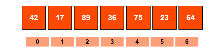

Multidimensional Arrays

These arrays have elements arranged in multiple dimensions, commonly visualized as tables with rows and columns. Elements are accessed using multiple indices.

PYTHON

matrix = [[1, 2, 3], [4, 5, 6], [7, 8, 9]]; print(matrix[1][2]) # Outputs: 6

C++

int matrix[3][3] = {{1, 2, 3}, {4, 5, 6}, {7, 8, 9}};

cout << matrix[1][2] << endl;  // Outputs: 6

JAVA

int[][] matrix = {{1, 2, 3}, {4, 5, 6}, {7, 8, 9}}; System.out.println(matrix[1][2]); // Outputs: 6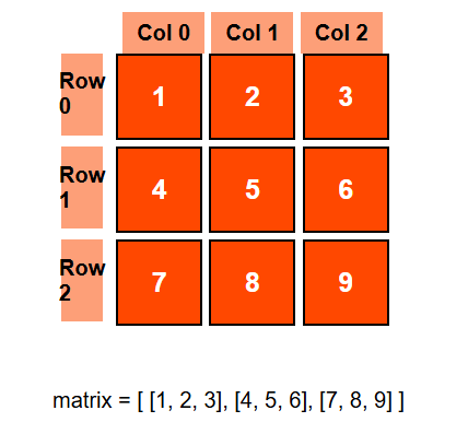

Array Representation

Memory Layout and Indexing

In memory, arrays are represented as consecutive blocks, with each block sized according to the data type. For example, if each integer requires 4 bytes of memory, an array of 5 integers would occupy 20 consecutive bytes.

The formula to calculate the memory address of an element at index i in a one-dimensional array is:

address = base_address + (i * size_of_data_type)

This formula explains why array access is so fast - it's a simple calculation rather than a search operation.

Animation HERE

Notation and Syntax in Various Programming Languages

Different programming languages have different ways to declare and use arrays:

PYTHON

fruits = ["apple", "banana", "cherry"]

C++

char fruits[3][10] = {"apple", "banana", "cherry"};

JAVA

String[] fruits = {"apple", "banana", "cherry"};

Array Initialization

Arrays can be initialized during declaration or element by element:

PYTHON

numbers = [1, 2, 3, 4, 5]

empty_array = []

empty_array.append(1)

empty_array.append(2)

C++

vector<int> numbers = {1, 2, 3, 4, 5};

vector<int> empty_array;

empty_array.push_back(1);

empty_array.push_back(2);

JAVA

int[] numbers = {1, 2, 3, 4, 5};

ArrayList<Integer> empty_array = new ArrayList<>();

empty_array.add(1);

empty_array.add(2);

Basic Operations on Arrays

Arrays support several core operations that form the basis of many algorithms and data manipulations. Let's focus on the four main operations: traversal, insertion, deletion, and searching.

Traversal in Arrays

Definition and Purpose

Traversal refers to visiting every element in the array once, typically to perform some operation on each element. Common traversal uses include:

Displaying all elements
Calculating sums or averages
Finding maximum/minimum values
Applying transformations to each element

Algorithm for Traversal

The basic algorithm for array traversal is straightforward:

Start from the first element (index 0)
Access the current element
Process the current element (display, calculate, transform, etc.)
Move to the next element
Repeat steps 2-4 until all elements are processed

Time Complexity of Traversal

Array traversal has a time complexity of O(n), where n is the number of elements in the array. This is because we must visit each element exactly once, and the time grows linearly with the array size.

Code Examples

Python

# ------------------- PYTHON -------------------
def traverse_array(arr):
    for i in range(len(arr)):
        print(f"Element at index {i}: {arr[i]}")

def traverse_for_each(arr):
    for element in arr:
        print(element)

C++

/* ------------------- C++ ------------------- */
#include <iostream>
#include <vector>
using namespace std;

void traverse_array(const vector<int>& arr) {
    for (int i = 0; i < arr.size(); i++) {
        cout << "Element at index " << i << ": " << arr[i] << endl;
    }

    // Using range-based for loop (alternative approach)
    for (int element : arr) {
        cout << element << endl;
    }
}

Java

/* ------------------- JAVA ------------------- */
public void traverseArray(int[] arr) {
    for (int i = 0; i < arr.length; i++) {
        System.out.println("Element at index " + i + ": " + arr[i]);
    }

    // Using enhanced for loop (alternative approach)
    for (int element : arr) {
        System.out.println(element);
    }
}

Insertion in Arrays

Definition and Scenarios

Insertion means adding an element to an array. Depending on where you want to add the element, insertion can be categorized into three types:

Insertion at the end
Insertion at the beginning
Insertion at a specific position

Insertion at the End

This is the simplest form of insertion, especially for dynamic arrays or array-like data structures that can resize themselves.

Python

# ------------------- PYTHON -------------------

def insert_at_end(arr, element):
    arr.append(element)
    return arr

numbers = [1, 2, 3, 4]
insert_at_end(numbers, 5)  # [1, 2, 3, 4, 5]

C++

/* ------------------- C++ ------------------- */
#include <vector>
using namespace std;

void insert_at_end(vector<int>& arr, int element) {
    arr.push_back(element);
}

vector<int> numbers = {1, 2, 3, 4};
insert_at_end(numbers, 5);  // {1, 2, 3, 4, 5}

Java

/* ------------------- JAVA ------------------- */
import java.util.ArrayList;

public void insertAtEnd(ArrayList<Integer> arr, int element) {
    arr.add(element);
}

ArrayList<Integer> numbers = new ArrayList<>();
numbers.add(1);
numbers.add(2);
numbers.add(3);
numbers.add(4);
insertAtEnd(numbers, 5);  // [1, 2, 3, 4, 5]

Insertion at the Beginning

Python

# ------------------- PYTHON -------------------

def insert_at_beginning(arr, element):
    arr.insert(0, element)
    return arr

numbers = [1, 2, 3, 4]
insert_at_beginning(numbers, 0)  # [0, 1, 2, 3, 4]

C++

/* ------------------- C++ ------------------- */
#include <vector>
using namespace std;

void insert_at_beginning(vector<int>& arr, int element) {
    arr.insert(arr.begin(), element);
}

vector<int> numbers = {1, 2, 3, 4};
insert_at_beginning(numbers, 0);  // {0, 1, 2, 3, 4}

Java

/* ------------------- JAVA ------------------- */
import java.util.ArrayList;

public void insertAtBeginning(ArrayList<Integer> arr, int element) {
    arr.add(0, element);
}

ArrayList<Integer> numbers = new ArrayList<>();
numbers.add(1);
numbers.add(2);
numbers.add(3);
numbers.add(4);
insertAtBeginning(numbers, 0);  // [0, 1, 2, 3, 4]

Insertion at a Specific Position

Python

# ------------------- PYTHON -------------------

def insert_at_position(arr, element, position):
    if position < 0 or position > len(arr):
        print("Invalid position")
        return arr
    arr.insert(position, element)
    return arr

numbers = [10, 20, 30, 40, 50]
insert_at_position(numbers, 25, 2)  # [10, 20, 25, 30, 40, 50]

C++

/* ------------------- C++ ------------------- */
#include <iostream>
#include <vector>
using namespace std;

void insert_at_position(vector<int>& arr, int element, int position) {
    if (position < 0 || position > arr.size()) {
        cout << "Invalid position" << endl;
        return;
    }
    arr.insert(arr.begin() + position, element);
}

vector<int> numbers = {10, 20, 30, 40, 50};
insert_at_position(numbers, 25, 2);  // {10, 20, 25, 30, 40, 50}

Java

/* ------------------- JAVA ------------------- */
import java.util.ArrayList;

public void insertAtPosition(ArrayList<Integer> arr, int element, int position) {
    if (position < 0 || position > arr.size()) {
        System.out.println("Invalid position");
        return;
    }
    arr.add(position, element);
}

ArrayList<Integer> numbers = new ArrayList<>();
numbers.add(10);
numbers.add(20);
numbers.add(30);
numbers.add(40);
numbers.add(50);
insertAtPosition(numbers, 25, 2);  // [10, 20, 25, 30, 40, 50]

Time Complexity Analysis

Insertion at the end: O(1) amortized for dynamic arrays
Insertion at the beginning or at a specific position: O(n) because it requires shifting elements

Deletion in Arrays

Definition and Scenarios

Deletion involves removing an element from an array. Like insertion, deletion can happen at the end, beginning, or at a specific position.

Deletion from the End

This is typically the most efficient deletion operation.

Python

# ------------------- PYTHON -------------------

def delete_from_end(arr):
    if len(arr) > 0:
        last_element = arr.pop()
        return last_element
    return None  # Array is empty

C++

/* ------------------- C++ ------------------- */
#include <vector>
using namespace std;

int delete_from_end(vector<int>& arr) {
    if (!arr.empty()) {
        int last_element = arr.back();
        arr.pop_back();
        return last_element;
    }
    return -1;  // Array is empty
}

Java

/* ------------------- JAVA ------------------- */
import java.util.ArrayList;

public Integer deleteFromEnd(ArrayList<Integer> arr) {
    if (!arr.isEmpty()) {
        return arr.remove(arr.size() - 1);  // Returns removed element
    }
    return null;  // Array is empty
}

Deletion from a Specified Position

When deleting from a specific position, all elements after that position need to be shifted to the left.

Python

# ------------------- PYTHON -------------------

def delete_from_position(arr, position):
    if position < 0 or position >= len(arr):
        print("Invalid position")
        return None
    deleted = arr[position]
    for i in range(position, len(arr) - 1):
        arr[i] = arr[i + 1]
    arr.pop()
    return deleted

C++

/* ------------------- C++ ------------------- */
#include <vector>
#include <iostream>
using namespace std;

int delete_from_position(vector<int>& arr, int position) {
    if (position < 0 || position >= arr.size()) {
        cout << "Invalid position" << endl;
        return -1;
    }
    int deleted = arr[position];
    for (int i = position; i < arr.size() - 1; i++) {
        arr[i] = arr[i + 1];
    }
    arr.pop_back();
    return deleted;
}

Java

/* ------------------- JAVA ------------------- */
import java.util.ArrayList;

public Integer deleteFromPosition(ArrayList<Integer> arr, int position) {
    if (position < 0 || position >= arr.size()) {
        System.out.println("Invalid position");
        return null;
    }
    int deleted = arr.get(position);
    for (int i = position; i < arr.size() - 1; i++) {
        arr.set(i, arr.get(i + 1));
    }
    arr.remove(arr.size() - 1);
    return deleted;
}

Time Complexity Analysis

Deletion from the end: O(1)
Deletion from the beginning or a specific position: O(n) due to shifting elements

Searching in Arrays

Definition and Use Cases

Searching involves finding an element in an array. Common use cases include checking if an element exists, finding its index, or counting occurrences.

Types of Searching Algorithms

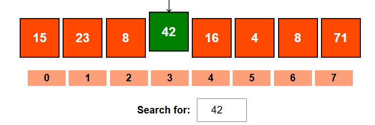
Linear Search

Linear search checks each element sequentially until it finds the target or reaches the end of the array. It works on both sorted and unsorted arrays.

Consider example - > [15, 23, 8, 42, 16, 4, 8, 71]

Python

# ------------------- PYTHON -------------------

def linear_search(arr, target):
    for i in range(len(arr)):
        # Check if target is present at i
        if arr[i] == target:
            return i
    # Target not found
    return -1

C++

/* ------------------- C++ ------------------- */
#include <vector>
using namespace std;

int linear_search(const vector<int>& arr, int target) {
    for (int i = 0; i < arr.size(); i++) {
        // Check if target is present at i
        if (arr[i] == target)
            return i;
    }
    // Target not found
    return -1;
}

Java

/* ------------------- JAVA ------------------- */
public int linearSearch(int[] arr, int target) {
    for (int i = 0; i < arr.length; i++) {
        // Check if target is present at i
        if (arr[i] == target)
            return i;
    }
    // Target not found
    return -1;
}

Time complexity: O(n) - In the worst case, we need to check every element.

Binary Search (for Sorted Arrays)

Binary search is much faster but requires the array to be sorted. It repeatedly divides the search interval in half.

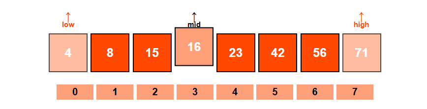
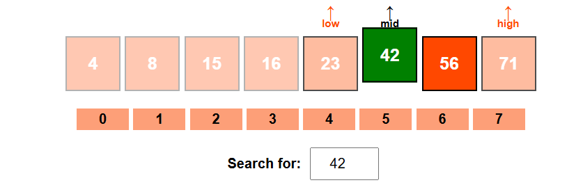
<visualization-box>

Implementation

Python

# ------------------- PYTHON -------------------

def binary_search(arr, target):
    left, right = 0, len(arr) - 1

    while left <= right:
        mid = (left + right) // 2

        # Check if target is present at mid
        if arr[mid] == target:
            return mid

        # If target is greater, ignore left half
        elif arr[mid] < target:
            left = mid + 1

        # If target is smaller, ignore right half
        else:
            right = mid - 1

    # Target not found
    return -1

C++

/* ------------------- C++ ------------------- */
#include <vector>
using namespace std;

int binary_search(const vector<int>& arr, int target) {
    int left = 0, right = arr.size() - 1;

    while (left <= right) {
        int mid = left + (right - left) / 2;

        // Check if target is present at mid
        if (arr[mid] == target)
            return mid;

        // If target is greater, ignore left half
        if (arr[mid] < target)
            left = mid + 1;

        // If target is smaller, ignore right half
        else
            right = mid - 1;
    }

    // Target not found
    return -1;
}

Java

/* ------------------- JAVA ------------------- */
public int binarySearch(int[] arr, int target) {
    int left = 0, right = arr.length - 1;

    while (left <= right) {
        int mid = left + (right - left) / 2;

        // Check if target is present at mid
        if (arr[mid] == target)
            return mid;

        // If target is greater, ignore left half
        if (arr[mid] < target)
            left = mid + 1;

        // If target is smaller, ignore right half
        else
            right = mid - 1;
    }

    // Target not found
    return -1;
}

Time complexity: O(log n) - With each step, we eliminate half of the remaining elements.

Time and Space Complexity Comparisons

Practical Considerations and Limitations

Limitations of Static Arrays

Static arrays, once created, have fixed sizes that cannot be changed. This leads to several limitations:

Fixed Size

If you need to add more elements than the array can hold, you must create a new, larger array and copy all elements.

// C++ example showing the limitation of fixed size

#include <iostream>
using namespace std;

int main() {
    int arr[5] = {1, 2, 3, 4, 5};

    // This will cause an array overflow and might crash the program
    // or lead to unexpected behavior
    arr[5] = 6;  // Trying to add a 6th element to a 5-element array

    return 0;
}

Costly Insert/Delete Operations

As we've seen, insertion and deletion operations (except at the end) require shifting elements, which is inefficient for large arrays.

Dynamic Arrays and Language-specific Details

Many modern programming languages provide dynamic arrays that can grow or shrink as needed:

Python lists
Java's ArrayList
C++'s vector

These dynamic structures handle memory allocation automatically but may have performance implications during resizing operations.

Best Practices for Efficient Array Usage

When you know the size in advance, pre-allocate the array to avoid costly resizing.
For frequent insertions/deletions at the beginning, consider using different data structures like linked lists.
For searching in large datasets, keep arrays sorted and use binary search.
Be aware of language-specific optimizations and built-in methods.

Conclusion
Arrays form the foundation of many data structures and algorithms. We've covered the four essential operations on arrays:
• Traversal: Visiting each element, usually in O(n) time
• Insertion: Adding elements at various positions, with implications for time complexity
• Deletion: Removing elements, also with varying complexity based on position
• Searching: Finding elements using linear or binary search techniques

Each operation has its own trade-offs regarding time and space complexity. Understanding these operations and their performance characteristics helps in choosing the right approach for your specific programming needs.

Arrays are ideal when you need random access to elements or when you're dealing with a fixed collection of items. However, for scenarios requiring frequent insertions or deletions, especially at the beginning or middle, other data structures might be more suitable.

As you continue learning about data structures, arrays will remain a key building block upon which more complex structures are built.

FAQs

Compare

vs InterviewCopilot.io

vs Interviews.chat

vs PrepAI

Resources

Blog

Success Stories

Help Center

Legal

Terms & Conditions

Cookie Policy

GDPR

Arrays: Essential Operations & Implementation Guide

Array Fundamentals

Characteristics of Arrays

Homogeneous Elements

Contiguous Memory Allocation

Types of Arrays

One-dimensional Arrays

Python

C++

JAVA

Multidimensional Arrays

PYTHON

C++

JAVA

Array Representation

Memory Layout and Indexing

Animation HERE

Notation and Syntax in Various Programming Languages

PYTHON

C++

JAVA

PYTHON

C++

JAVA

Basic Operations on Arrays

Traversal in Arrays

Definition and Purpose

Algorithm for Traversal

Time Complexity of Traversal

Code Examples

Python

C++

Java

Insertion in Arrays

Definition and Scenarios

Insertion at the End

Python

C++

Java

Insertion at the Beginning

Python

C++

Java

Insertion at a Specific Position

Python

C++

Java

Time Complexity Analysis

Deletion in Arrays

Definition and Scenarios

Deletion from the End

Python

C++

Java

Deletion from a Specified Position

Python

C++

Java

Time Complexity Analysis

Searching in Arrays

Definition and Use Cases

Types of Searching Algorithms

Linear Search

Python

C++

Java

Binary Search (for Sorted Arrays)

Implementation

Python

C++

Java

Time and Space Complexity Comparisons

Practical Considerations and Limitations

Limitations of Static Arrays

Fixed Size

Costly Insert/Delete Operations

Dynamic Arrays and Language-specific Details

Best Practices for Efficient Array Usage

FAQs

TAGS